
The roster worked for a month. Pick a department in one column, and the next column only offered that department’s people. Then someone inserted a row for a new starter, and their second dropdown offered nothing at all. Nobody changed a formula. Nobody touched the list. It just stopped.
If that sounds familiar, you built a dependent dropdown in Google Sheets the way every tutorial shows, and you hit the part the tutorials skip. This post rebuilds that setup in a test sheet, inserts a row, shows exactly what breaks and why, and then gives you three ways to stop it happening, from a formula change to a free add-on I built for this exact problem. Everything below was run live while writing, and the screenshots are the proof.
Table of Contents
The short answer
A dependent dropdown in Google Sheets needs a helper cell for every row, because Sheets has no native way to make one dropdown depend on another. When you insert a row, Sheets copies the dropdown to the new row but not the helper formula, so the new dropdown points at an empty cell and offers an empty list.
The fixes: build the helper as one formula that covers the whole column, copy cells from a working row instead of inserting a blank one, or use an add-on that writes each row’s list for you and rebuilds it on demand.
How the usual dependent dropdown is built
Google’s own dropdown help page lists two kinds of dropdown: a fixed list, and “Dropdown (from a range)”. Neither can depend on another cell. So every dependent dropdown you have ever seen is a workaround built from three parts:
- A category and option list. Wine, Red. Wine, White. Spirits, Whisky. One pair per row.
- A helper cell for each entry row that works out which options belong to the category picked in that row. Some tutorials use a named range per category and INDIRECT; the one below uses FILTER, which needs no named ranges. Either way it is one helper per row.
- A “Dropdown (from a range)” rule on the option column that points at the helper.
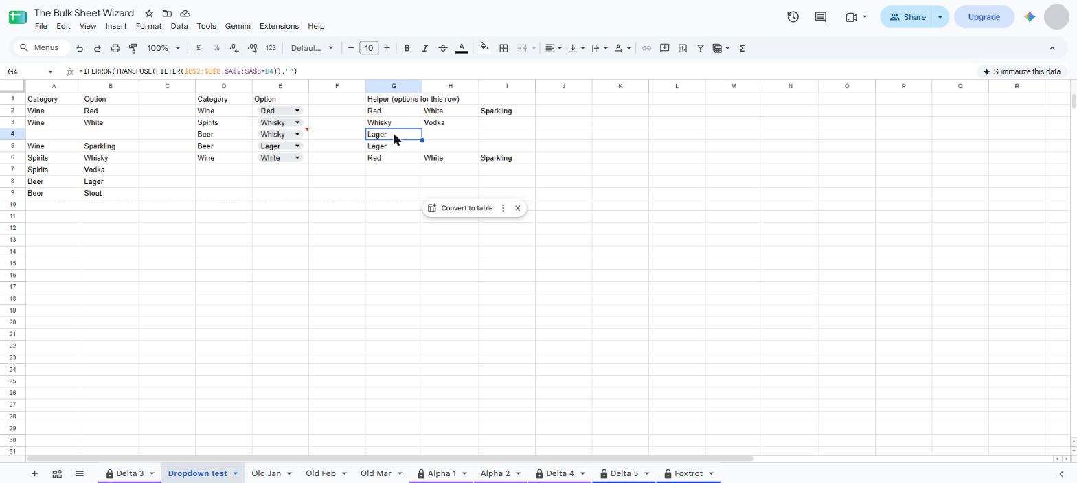
Here is the FILTER version, which is the one I tested. Column D is the category the person picks, column E is the option dropdown, and G2 holds the helper for row 2:
=IFERROR(TRANSPOSE(FILTER($B$2:$B$7, $A$2:$A$7=D2)), "")Copy that down one row per entry row. Then select the option cells, open Data › Data validation, choose “Dropdown (from a range)” and enter =G2:L2 with no dollar signs. That is the trick most tutorials leave out: Sheets shifts a relative range for each cell in the rule, so E3 reads G3:L3, E4 reads G4:L4, and one rule covers the lot. The panel’s own tip says to use absolute references to lock rows, which is a polite way of saying unlocked ones move.
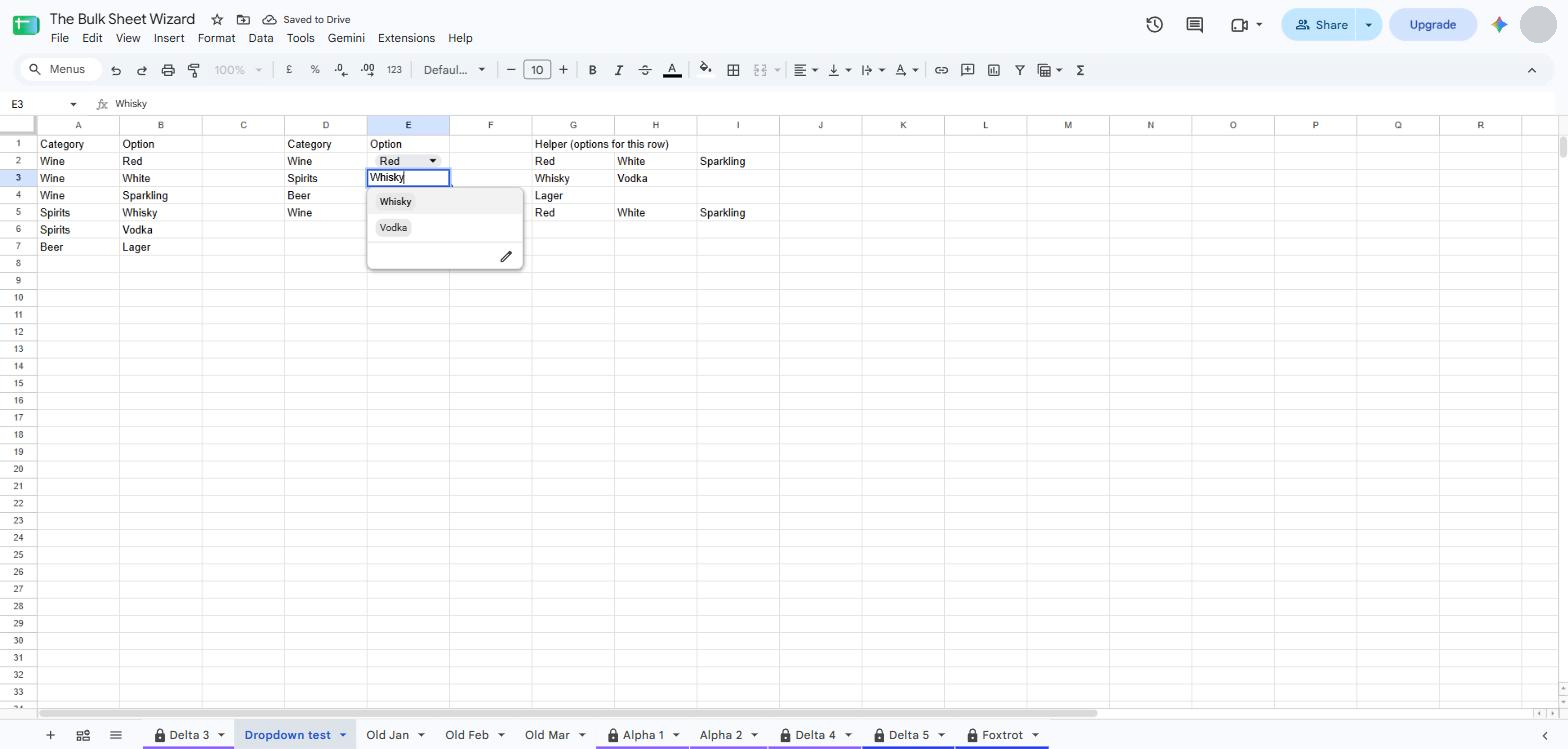
At this point it works. Pick Spirits in D3 and E3 offers Whisky and Vodka, nothing else. The helper row is doing the thinking, and the dropdown is just reading it.
What happens when you insert a row
I right-clicked row 4 and chose Insert 1 row above, then typed Spirits into the new row’s category cell and opened its option dropdown. This is what came up.
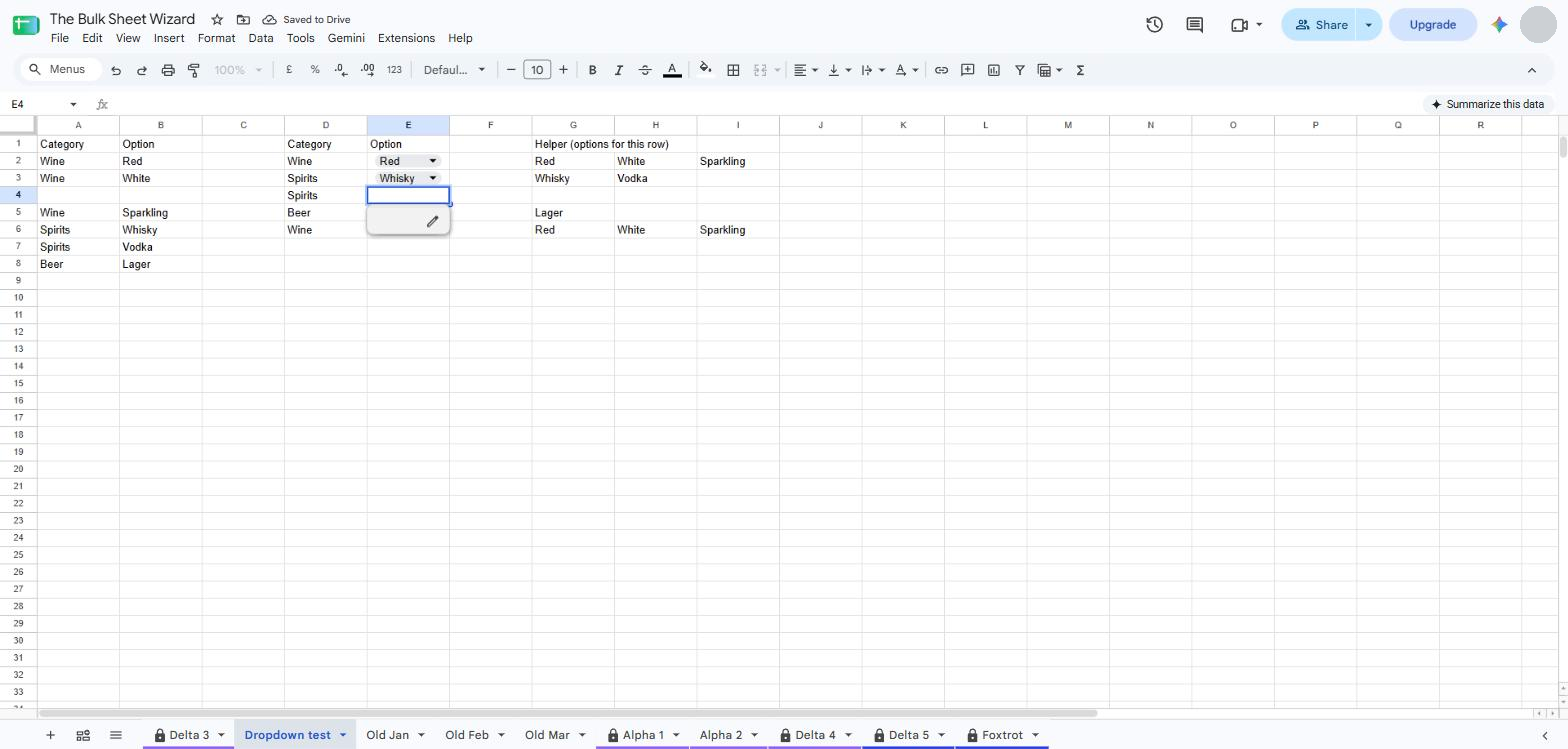
The dropdown arrow is there, so it looks fine at a glance. The list behind it is empty. Sheets treats data validation as formatting, and inserted rows inherit formatting from the row above, so the new row got a rule pointing at G4:L4. It did not inherit the helper formula, because formulas are content, not formatting, and G4 is blank. An empty helper means an empty list.
That is the whole failure in one sentence: the rule travels, the formula does not. And because the dropdown arrow still shows, the person filling in the roster assumes the sheet is broken rather than the row.
Three more things went wrong in the same test, and they are worth knowing before you go looking for a fix:
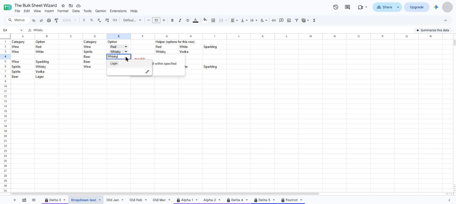
- A copied row keeps its old answer. Copying the cells from a working row is the usual repair, and it does bring the helper along. But if you then change the category, the old option stays in the cell with a red corner and an “Invalid” warning. It does not clear itself.
- Copying a whole row can corrupt your list. If the category list lives on the same sheet as the entries, copying an entire row copies a list row too. I did it once by accident and gave the Wine category a second “White”.
- New options at the bottom of the list vanish. The helper formula uses a fixed range,
$A$2:$A$7. Add a new pair below the last row and the range does not grow to include it. I added Beer, Stout on row 9 and the Beer rows kept offering Lager alone.
The INDIRECT and named range version has all of the above plus its own list: a named range per category, names that cannot contain spaces without being cleaned up, and a new named range every time you add a category. Sheets Bootcamp’s guide is honest about it: “Each row needs its own helper”, and it calls that “the real cost of the technique”.
Three ways to stop it breaking
1. One helper formula for the whole column
Instead of one FILTER per row, put a single MAP formula at the top of the helper column and let it produce a list for every row at once, blank rows included. Use whole-column references for the list, so new options at the bottom count too.
=MAP(D2:D20, LAMBDA(c, IF(c="",, TOROW(FILTER($B$2:$B, $A$2:$A=c)))))Read it as: for each category cell in D2 to D20, if it is blank give nothing, otherwise lay that category’s options out across the row. I ran this in the test sheet and it produced the right list on every row, including Stout for the Beer rows that the fixed-range version had missed. Extend D2:D20 to cover as many rows as you will ever need, and set the validation rule on the same rows with the relative range trick from earlier.
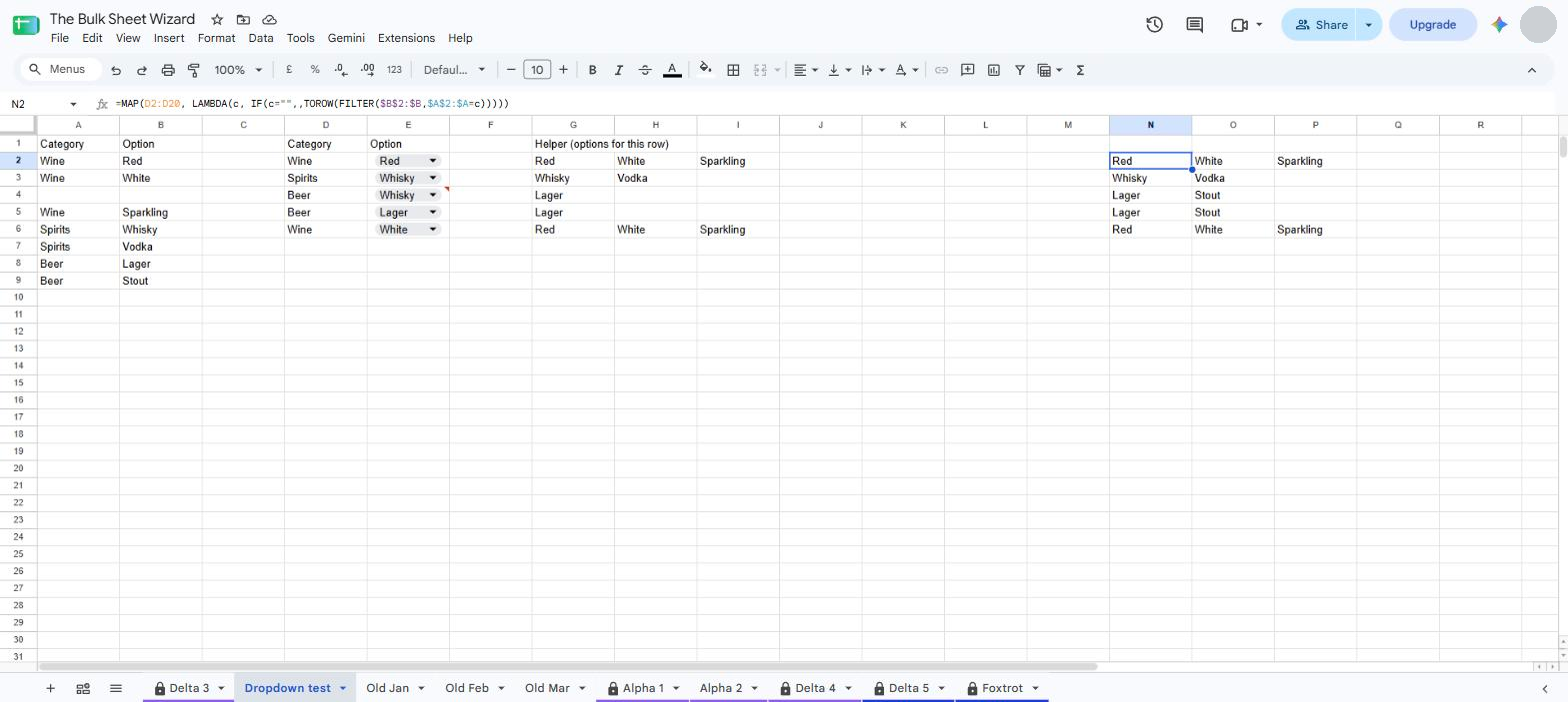
The cost: it is one formula doing every row’s work, so it recalculates whenever the list or the category column changes, and a long sheet can feel slower for it. And because the whole column comes from one cell, anyone who types over that cell takes every row’s list down at once. Keep the helper on a separate tab and tell people not to touch it.
2. Copy a row, never insert a blank one
If you would rather not change the build, change the habit. To add a row, select the cells of a working row (the category, the option and its helper, not the whole row), copy, and paste into the new row. The helper comes with them and adjusts itself. Then clear the option cell before picking a category, so you do not carry the old answer across with its red corner.
This works. It also depends on every person who ever edits the sheet remembering it, which is why it usually holds until the second new starter.
3. Let an add-on write the lists
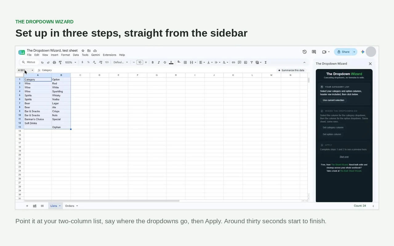
This is the one I built, so weigh it accordingly. The Dropdown Wizard takes the same two-column list and writes each row’s option list into the dropdown rule directly, so there are no helper cells, no named ranges and no INDIRECT anywhere in the sheet. Three steps in a sidebar:
- Select your category and option list, header row included, and click Use current selection.
- On the tab where people type, select the category cells and click Set category column, then the option cells and click Set option column.
- Check the preview, then Apply. If those cells already carry a validation rule the add-on did not write, it stops and asks before replacing it.
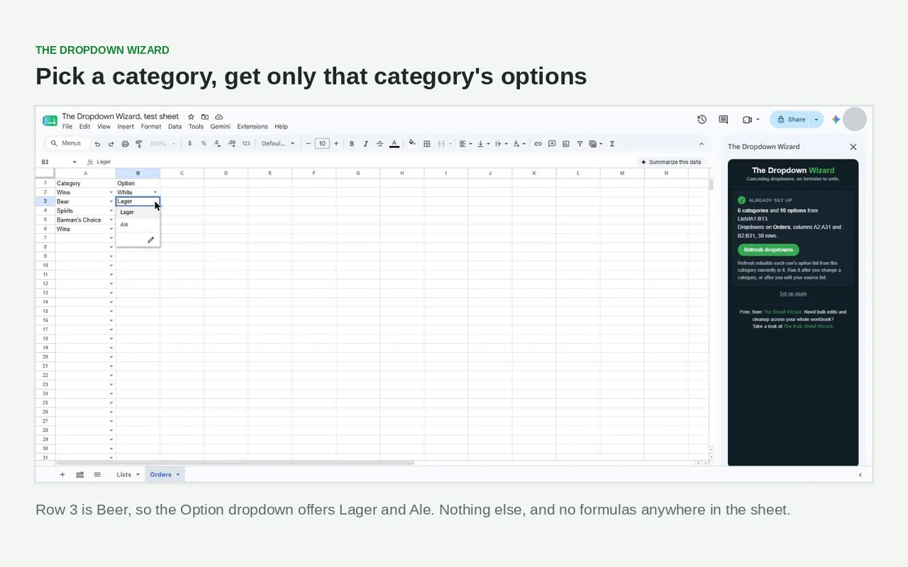
Pick Beer in a row and the option cell beside it offers Lager and Ale. Nothing else, and no formulas anywhere in the sheet.
Now the honest part. The lists are built from your category list at the moment you press Apply, and from whatever category is sitting in each row at that moment. They are not live. Add an option, fix a spelling, change a row’s category, or add rows, and the dropdowns keep offering the old choices until you run Extensions › The Dropdown Wizard › Refresh dropdowns. That takes about two seconds and anyone with the file open can do it, but it is the one thing to remember, and the help page says so in bold. That trade is what lets the add-on work with the narrow “this spreadsheet only” permission and stay free, with no account and no card.
Keep the list, not the machinery
Whichever fix you pick, the thing worth protecting is the list. A long two-column list, category then option, one pair per row, is the shape all three fixes read from, it is easy to hand to someone else, and it survives being sorted, filtered and added to. The wide layout most tutorials start with, one column per category with the options stacked under it, is the shape that runs out of room and needs a new column, a new named range and a new formula every time the business adds a category. Build the list long, put it on its own tab, and the machinery, whichever kind you choose, has something stable to stand on.
Frequently asked questions
Does Google Sheets have a built-in dependent dropdown?
No. Google’s dropdown options are a fixed list or a list from a range, and neither can change based on another cell. Every dependent dropdown in Google Sheets is a workaround built from a helper cell, a formula and a validation rule, or an add-on that writes the rules for you.
Why will Google Sheets not accept INDIRECT in the data validation box?
The “Dropdown (from a range)” field wants a range, not a formula. Type =INDIRECT(D2) into it and Sheets answers “Please enter a valid range”, so INDIRECT has to live in a helper cell and the rule points at the helper. That is why every tutorial ends up with a helper column, and why the helper is the part that goes missing when rows are inserted.
Why is my dependent dropdown empty in a new row?
Because the new row inherited the validation rule from the row above but not the helper formula. The rule points at a blank helper cell, so the list is empty. Copy the helper cell from a working row, or switch to a helper built with one whole-column formula so every row is covered.
How do I add a new category or option?
Add the pair to your list. With a fixed-range helper you then have to widen the range; with whole-column references or a MAP helper it is picked up on its own. With The Dropdown Wizard, add the pair and run Refresh dropdowns.
Do I need a helper column at all?
For a formula-based build, yes, one way or another, because Sheets cannot evaluate a formula inside the dropdown rule. The only way to have no helper cells in the sheet is to have something write each row’s list into the rule itself, which is what the add-on does, at the price of needing a Refresh when the list changes.
One list, three clicks
Dependent dropdowns break on new rows because the helper does not travel with the rule. Fix the helper, fix the habit, or hand the job to something that writes the rules for you. If you want the third option, install The Dropdown Wizard from the Google Workspace Marketplace, point it at your list, and try it on the tab that keeps breaking. It is free, and the whole setup takes about thirty seconds.